AdvancedTop, Main, Index
This section provides advanced examples from the examples folder in the root directory of SpiceGenTcl. Rather than focusing on basic operations, we highlight advanced use cases that showcase the full capabilities of both the package and the Tcl language. List of availible examples:
- Monte-Carlo simulation - "examples/ngspice/advanced/monte_carlo.tcl" and "examples/xyce/advanced/monte_carlo.tcl" file
- Parameters extraction of diode model parameters - "examples/ngspice/advanced/diode_extract.tcl" file
- Inverter performance optimization - "examples/ngspice/advanced/inverter_optimization.tcl" file
Monte-Carlo simulationTop, Main, Index
This example demonstrates multiple runs of a simple filter circuit and the collection of the resulting statistical distribution of frequency bandwidths. The original circuit source is from the ngspice source distribution. The target filter circuit is:
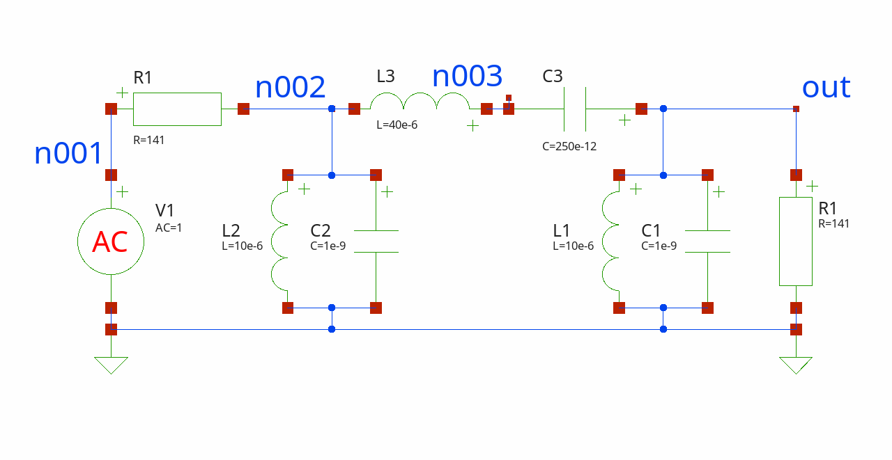
The filter is a 3rd-order Chebyshev bandpass. The first step is to build the circuit and obtain the magnitude of the transfer characteristic:
# create top-level circuit
set circuit [Circuit new {Monte-Carlo}]
# add elements to circuit
$circuit add [Vac new 1 n001 0 -ac 1]
$circuit add [R new 1 n002 n001 -r 141]
$circuit add [R new 2 0 out -r 141]
C create c1 1 out 0 -c 1e-9
L create l1 1 out 0 -l 10e-6
C create c2 2 n002 0 -c 1e-9
L create l2 2 n002 0 -l 10e-6
C create c3 3 out n003 -c 250e-12
L create l3 3 n003 n002 -l 40e-6
foreach elem [list c1 l1 c2 l2 c3 l3] {
    $circuit add $elem
}
$circuit add [Ac new -variation oct -n 100 -fstart 250e3 -fstop 10e6]
#set simulator with default
set simulator [Batch new {batch1}]
# attach simulator object to circuit
$circuit configure -simulator $simulator
Here, we use a different method for creating a class instance: create instead of new. With create, we can directly set a custom object reference name, rather than relying on the automatically generated one by Tcl.
C create c1 1 out 0 -c 1e-9
Keep in mind that c1 is an object reference, not the name of a variable storing the reference. Therefore, it can be used as an object command directly, without the need for a $.
To calculate the magnitude of the transfer function in dB scale from the output voltage phasor, we create a procedure:
proc calcDbMag {re im} {
    set mag [= {sqrt($re*$re+$im*$im)}]
    set db [= {10*log($mag)}]
    return $db
}

proc calcDbMagVec {vector} {
    foreach value $vector {
        lappend db [calcDbMag [@ $value 0] [@ $value 1]]
    }
    return $db
}
calcDbMagVec | Procedure that apply calcDbMag to list of complex values. |
Run and plot the result:
# run simulation
$circuit runAndRead
# get data dictionary
set data [$circuit getDataDict]
set trace [calcDbMagVec [dget $data v(out)]]
set freqs [dget $data frequency]
foreach x $freqs y $trace {
    lappend xydata [list [@ $x 0] $y]
}
puts [findBW [lmap freq $freqs {@ $freq 0}] $trace -10]
set chartTransMag [ticklecharts::chart new]
$chartTransMag Xaxis -name "Frequency, Hz" -minorTick {show "True"} -type "log" -splitLine {show "True"}
$chartTransMag Yaxis -name "Magnitude, dB" -minorTick {show "True"} -type "value" -splitLine {show "True"}
$chartTransMag SetOptions -title {} -tooltip {trigger "axis"} -animation "False" -toolbox {feature {dataZoom {yAxisIndex "none"}}} -grid {left "10%" right "15%"} -backgroundColor "#212121"
$chartTransMag Add "lineSeries" -data $xydata -showAllSymbol "nothing" -symbolSize "1"
set fbasename [file rootname [file tail [info script]]]
$chartTransMag Render -outfile [file normalize [file join .. html_charts ${fbasename}_typ.html]] -width 1000px
We define pass bandwidth by edge values -10dB, to find them we use next procedure:
proc findBW {freqs vals trigVal} {
    # calculate bandwidth of results
    set bw [dget [measure -xname freqs -data [dcreate freqs $freqs vals $vals] -trig "-vec vals -val $trigVal -rise 1" -targ "-vec vals -val $trigVal -fall 1"] xdelta]
    return $bw
}
Find bandwidth:
puts [findBW [lmap freq $freqs {@ $freq 0}] $trace -10]
The value is 1.086255 Mhz.
Our goal is to obtain a distribution of bandwidths by varying the filter parameters. To generate random values for these parameters, we use the built-in functions of the math::statistics package from Tcllib. The parameters can be distributed either normally or uniformly. For uniform distribution, we use ::math::statistics::random-uniform xmin xmax number; for normal distribution, we use ::math::statistics::random-normal mean stdev number. For uniform distribution, we define the following min and max limits for each C and L element:
set distLimits [dcreate c1 [dcreate min 0.9e-9 max 1.1e-9] l1 [dcreate min 9e-6 max 11e-6] c2 [dcreate min 0.9e-9 max 1.1e-9] l2 [dcreate min 9e-6 max 11e-6] c3 [dcreate min 225e-12 max 275e-12] l3 [dcreate min 36e-6 max 44e-6]]
We can specify different numbers of simulations; the more runs we perform, the more accurate the representation becomes. For example, we set the number of simulations to 1,000 runs with 15 intervals for constructing a boxplot:
# set number of simulations
set mcRuns 100
set numOfIntervals 15
Now we ready to run simulations 1000 times and collect results:
# loop in which we run simulation with uniform distribution
for {set i 0} {$i<$mcRuns} {incr i} {
    #set elements values according to uniform distribution
    foreach elem [list c1 l1 c2 l2 c3 l3] {
        $elem actOnParam -set [string index $elem 0] [random-uniform {*}[dict values [dget $distLimits $elem]] 1]
    }
    # run simulation
    $circuit runAndRead
    # get data dictionary
    set data [$circuit getDataDict]
    # get results
    if {$i==0} {
        set freqs [dget $data frequency]
        foreach freq $freqs {
            lappend freqRes [@ $freq 0]
        }
    }
    # get vout frequency curve
    lappend traceListUni [calcDbMagVec [dget $data v(out)]]
    # calculate bandwidths values
    lappend bwsUni [findBW $freqRes [@ $traceListUni end] -10]
}
To obtain the distribution, we need to determine reasonable limits based on the minimum and maximum of the generated bandwidth values. Using the specified number of intervals (15), we apply the following procedure:
proc createIntervals {data numOfIntervals} {
    set intervals [::math::statistics::minmax-histogram-limits [tcl::mathfunc::min {*}$data]  [tcl::mathfunc::max {*}$data] $numOfIntervals]
    lappend intervalsStrings [format "<=%.2e" [@ $intervals 0]]
    for {set i 0} {$i<[- [llength $intervals] 1]} {incr i} {
        lappend intervalsStrings [format "%.2e-%.2e" [@ $intervals $i] [@ $intervals [+ $i 1]]]
    }
    return [dcreate intervals $intervals intervalsStr $intervalsStrings]
}
Here, we use the dedicated procedure from the statistics package: ::math::statistics::minmax-histogram-limits min max number. Additionally, we construct strings in form leftVal-rightVal that represent the intervals on the boxplot chart. We call this procedure and store the results:
set uniIntervals [createIntervals $bwsUni $numOfIntervals]
Finally, to obtain the expected histogram for a uniform distribution, we use the following procedure with the built-in function: ::math::statistics::histogram-uniform xmin xmax limits number:
proc createDist {data intervals} {
    set dist [::math::statistics::histogram $intervals $data]
    return [lrange $dist 0 end-1]
}
Call the createDist procedure to calculate the histogram y-axis values, which correspond to the number of bandwidths within each interval:
set normDist [createDist $bwsNorm [dget $normIntervals intervals]]
The same sequence of steps is applied for the normal distribution. We assume that std = (xmax - xmin) / 6, where xmax and xmin are the limits of the uniform distribution.
# set parameter's normal distributions limits
set normalLimits [dcreate c1 [dcreate mean 1e-9 std [/ 0.1e-9 3]] l1 [dcreate mean 10e-6 std [/ 1e-6 3]] c2 [dcreate mean 1e-9 std [/ 0.1e-9 3]] l2 [dcreate mean 10e-6 std [/ 1e-6 3]] c3 [dcreate mean 250e-12 std [/ 25e-12 3]] l3 [dcreate mean 40e-6 std [/ 4e-6 3]]]

## loop in which we run simulation with normal distribution
for {set i 0} {$i<$mcRuns} {incr i} {
    #set elements values according to normal distribution
    foreach elem [list c1 l1 c2 l2 c3 l3] {
        $elem $elem actOnParam -set [string index $elem 0] [random-normal {*}[dict values [dget $normalLimits $elem]] 1]
    }
    # run simulation
    $circuit runAndRead
    # get data dictionary
    set data [$circuit getDataDict]
    # get results
    if {$i==0} {
        set freqs [dget $data frequency]
        foreach freq $freqs {
            lappend freqRes [@ $freq 0]
        }
    }
    # get vout frequency curve
    lappend traceListNorm [calcDbMagVec [dget $data v(out)]]
    # calculate bandwidths values
    lappend bwsNorm [findBW $freqRes [@ $traceListNorm end] -10]
}
# get distribution of bandwidths with normal parameters distribution
set normIntervals [createIntervals $bwsNorm $numOfIntervals]
set normDist [createDist $bwsNorm [dget $normIntervals intervals]]
Finally, we plot resulted distributions:
# plot results with ticklecharts
# chart for uniformly distributed parameters
set chartUni [ticklecharts::chart new]
$chartUni Xaxis -name "Frequency intervals, Hz" -data [list [dget $uniIntervals intervalsStr]] -axisTick {show "True" alignWithLabel "True"} -axisLabel {interval "0" rotate "45" fontSize "8"}
$chartUni Yaxis -name "Bandwidths per interval" -minorTick {show "True"} -type "value"
$chartUni SetOptions -title {} -tooltip {trigger "axis"} -animation "False" -toolbox {feature {dataZoom {yAxisIndex "none"}}} -backgroundColor "#212121"
$chartUni Add "barSeries" -data [list $uniDist]
# chart for normally distributed parameters
set chartNorm [ticklecharts::chart new]
$chartNorm Xaxis -name "Frequency intervals, Hz" -data [list [dget $normIntervals intervalsStr]] -axisTick {show "True" alignWithLabel "True"} -axisLabel {interval "0" rotate "45" fontSize "8"}
$chartNorm Yaxis -name "Bandwidths per interval" -minorTick {show "True"} -type "value"
$chartNorm SetOptions -title {} -tooltip {trigger "axis"} -animation "False" -toolbox {feature {dataZoom {yAxisIndex "none"}}} -backgroundColor "#212121"
$chartNorm Add "barSeries" -data [list $normDist]
# create multiplot
set layout [ticklecharts::Gridlayout new]
$layout Add $chartNorm -bottom "10%" -height "35%" -width "75%"
$layout Add $chartUni -bottom "60%" -height "35%" -width "75%"

set fbasename [file rootname [file tail [info script]]]
$layout Render -outfile [file normalize [file join .. html_charts $fbasename.html]] -height 800px -width 1200px
We can clearly see the difference between normal and uniform distributions; the intervals are close due to setting the standard deviation of the normal distribution as std = (xmax - xmin) / 6.
We can also take the uniform intervals and calculate the normal distribution values at these intervals:
# find distribution of normal distributed values in uniform intervals
set normDistWithUniIntervals [createDist $bwsNorm [dget $uniIntervals intervals]]
set chartCombined [ticklecharts::chart new]
$chartCombined Xaxis -name "Frequency intervals, Hz" -data [list [dget $uniIntervals intervalsStr]] -axisTick {show "True" alignWithLabel "True"} -axisLabel {interval "0" rotate "45" fontSize "8"}
$chartCombined Yaxis -name "Bandwidths per interval" -minorTick {show "True"} -type "value"
$chartCombined SetOptions -title {} -legend {} -tooltip {trigger "axis"} -animation "False" -toolbox {feature {dataZoom {yAxisIndex "none"}}} -grid {left "10%" right "15%"} -backgroundColor "#212121"
$chartCombined Add "barSeries" -data [list $uniDist] -name "Uniform"
$chartCombined Add "barSeries" -data [list $normDistWithUniIntervals] -name "Normal"
$chartCombined Render -outfile [file normalize [file join .. html_charts ${fbasename}_combined.html]] -height 800px -width 1200px
Parameters extraction of diode model parametersTop, Main, Index
In this advanced example we will do curve fitting procedure to extract parameters of diode model. We use measured (emulated with more advanced diode model generated data, with added small distorsion and make non-equal voltage steps) forward current characteristic of diode.
This example demands two additional Tcl packages to make fast interpolation and Levenberg-Marquardt optimization algorithm:
Also, the tclcsv package is used for data reading.
The main steps of this procedure are:
- Create cost function that calculates difference between simulated and measured data, and which should be minimized
- Select the region of optimization
- Set list of parameters that will be extracted, define lower and upper limits for them.
- Run optimization
- Use resulted values as initial values for next optimization in different region
- ...
- Repeat until the quality of fitting reaches required level.
First step is to define the cost function that will be used by the optimizer:
proc diodeIVcalc {xall pdata args} {
    dict with pdata {}
    $model actOnParam -set is [@ $xall 0] n [@ $xall 1] rs [@ $xall 2] ikf [@ $xall 3]
    $vSrc actOnParam -set start $vMin stop $vMax incr $vStep
    $circuit runAndRead
    set data [$circuit getDataDict]
    foreach iVal $i iSim [lmap i [dget $data i(va)] {= {-$i}}] {
        lappend fvec [= {log(abs($iVal))-log(abs($iSim))}]
        lappend fval $iSim
    }
    return [dcreate fvec $fvec fval $fval]
}
The input arguments are:
xall- list with fitting parameters, in our case, the parameters of the diode model.pdata- the dictionary containing information that allows to calculate cost function, in our case it contains multiple fields that will be explained below.args- any additional arguments, usually is used for passing information for calculating analytic derivatives.
Let me expand the values in pdata dictionary:
v- list of applied voltages valuesi- list of measured current valuescircuit- top circuit object simulating forward diode currentmodel- diode model objectvMin- start of the voltage regionvMax- end of the voltage regionvStep- size of voltage stepvSrc- voltage source object
First line creates variables with the same name as keys of pdata dictionary:
dict with pdata {}
Then we set parameters values of the diode model object using ::SpiceGenTcl::Model::actOnParam method:
$model actOnParam -set is [@ $xall 0] n [@ $xall 1] rs [@ $xall 2] ikf [@ $xall 3]
The same we do with voltage source element:
$vSrc actOnParam -set start $vMin stop $vMax incr $vStep
Then we run circuit with new parameters and read data back to calculate residuals:
$circuit runAndRead
set data [$circuit getDataDict]
Calculating residuals and save simulated data in the loop:
foreach iVal $i iSim [lmap i [dget $data i(va)] {= {-$i}}] {
    lappend fvec [= {log(abs($iVal))-log(abs($iSim))}]
    lappend fval $iSim
}
The residuals is calculated with the next formula:
f = log ⎛|i    |⎞ - log ⎛|i   |⎞
        ⎝| meas|⎠       ⎝| sim|⎠
We use logarithm of values because the current values span across multiple orders, from 1e-8 to 1e-2, that creates issue for fitting algorithm.
Procedure returns dictionary that contains lists with residuals and diode current under the keys fvec and fval, and fvec key is mandatory because list under this key is used by optimization procedure.
To run simulation we need to build circuit and define necessary objects:
set diodeModel [DiodeModel new diomod -is 1e-12 -n 1.0 -rs 30 -cj0 1e-9 -trs1 0.001 -xti 5 -ikf 1e-4]
set vSrc [Dc new -src va -start 0 -stop 2 -incr 0.02]
set circuit [Circuit new {diode IV}]
$circuit add [D new 1 anode 0 -model diomod -area 1]
$circuit add [Vdc new a anode 0 -dc 0]
$circuit add $diodeModel
$circuit add $vSrc
set tempSt [Temp new 25]
$circuit add $tempSt
$circuit configure -simulator [Batch new {batch1}]
We save object references for diode model and voltage source into dedicated variable to use it in cost function - it will be saved into pdata dictionary.
Next, we read measured data from .csv file with tclcsv package:
set file [open [file join $fileDataPath iv25.csv]]
set ivTemp25 [csv_read -startline 1 $file]
close $file
set vRaw [lmap elem $ivTemp25 {@ $elem 0}]
set iRaw [lmap elem $ivTemp25 {@ $elem 1}]
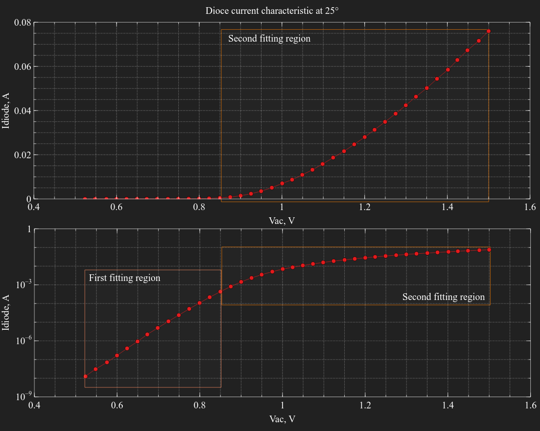
The loaded data is (with selected regions of fitting):
Fitting in first regionTop, Main, Index
First region we want to fit is the region of ideal diode, it spans from minimum voltage to approximately 0.85V. We set these limits in variables vMin, vMax and define the equal step of voltage vStep.
set vMin [min {*}$vRaw]
set vMax 0.85
set vStep 0.02
We use fixed voltage step instead of data points defined in measured data with non-equal steps to ease the defining the sweep of voltage in simulator - we can use DC sweep of voltage source with fixed step. So, we use linear interpolation to get values of current at even grid with defined minimum and maximum values. Then, we create pdata dictionary with corresponding values:
set vInterp [lseq $vMin to $vMax by $vStep]
set iInterp [lin1d -x $vRaw -y $iRaw -xi $vInterp]
set pdata [dcreate v $vInterp i $iInterp circuit $circuit model $diodeModel vMin $vMin vMax $vMax vStep $vStep vSrc $vSrc]
Command lin1d is imported from tclinterp package.
Parameters that we need to find (extract) are:
is | Saturation current. |
n | Ideality factor. |
rs | Series resistance. |
ikf | Forward knee current. |
In first region the parameters of interest are n and is0 - it affects current curve the most in this region.
Parameter are represented as special objects ::tclopt::ParameterMpfit from tclopt package, where we can define initial values and lower/upper limits:
set iniPars [list 1e-14 1.0 30 1e-4]
set par0 [::tclopt::ParameterMpfit new is [@ $iniPars 0] -lowlim 1e-17 -uplim 1e-12]
set par1 [::tclopt::ParameterMpfit new n [@ $iniPars 1] -lowlim 0.5 -uplim 2]
set par2 [::tclopt::ParameterMpfit new rs [@ $iniPars 2] -fixed -lowlim 1e-10 -uplim 100]
set par3 [::tclopt::ParameterMpfit new ikf [@ $iniPars 3] -fixed -lowlim 1e-12 -uplim 0.1]
For rs and ikf parameters we specify option -fixed to make them constant during the first region fitting.
Optimization is done with Levenberg-Marquardt algorithm based optimizator from tclopt package. First step is to create ::tclopt::Mpfit object that defines the optimization parameters:
set optimizer [::tclopt::Mpfit new -funct diodeIVcalc -m [llength $vInterp] -pdata $pdata]
The arguments we pass here are:
-funct | Name of the procedure calculating the residuals. |
-m | Number of fitting points. |
-pdata | Dictionary that is passed to cost function procedure. |
Then we add parameters to $optimizer object, and the order of adding them should match the order of the elements list xall we pass values to cost function:
$optimizer addPars $par0 $par1 $par2 $par3
Then we can run the simulation, read the resulted list of parameters x and print formatted values:
set result [$optimizer run]
set resPars [dget $result x]
puts [format "is=%.3e, n=%.3e, rs=%.3e, ikf=%.3e" {*}[dget $result x]]
The result is:
is=5.771e-17, n=1.050e+00, rs=3.000e+01, ikf=1.000e-04
You can notice that is and n now have different values, and rs and ikf remains the same because of -fixed option.
Fitting in second regionTop, Main, Index
Now we are ready to fit curve in the second ohmic/high-injection region. It started at the upper end of first region and continue until the end of the data. We interpolate this range with the same voltage step:
set vMin 0.85
set vMax [max {*}$vRaw]
set vInterp [lseq $vMin to $vMax by $vStep]
set iInterp [lin1d -x $vRaw -y $iRaw -xi $vInterp]
We will use the same pdata variable containing dictionary, but change the current and voltage data and limits:
dset pdata v $vInterp
dset pdata i $iInterp
dset pdata vMin $vMin
dset pdata vMax $vMax
We make is and n parameters fixed this time, and free the rs and ikf:
$par0 configure -fixed 1 -initval [@ $resPars 0]
$par1 configure -fixed 1 -initval [@ $resPars 1]
$par2 configure -fixed 0
$par3 configure -fixed 0
You can notice that we supply the resulted values of is and n as the initial values to the second fitting, so we have two parameters already fitted before start the next optimization.
Replace $optimizer object fields with the new values:
$optimizer configure -m [llength $vInterp] -pdata $pdata
Run, read result and print new parameters values:
set result [$optimizer run]
set fittedIdiode [dget [diodeIVcalc [dget $result x] $pdata] fval]
set resPars [dget $result x]
puts [format "is=%.3e, n=%.3e, rs=%.3e, ikf=%.3e" {*}[dget $result x]]
The result is:
is=5.771e-17, n=1.050e+00, rs=5.430e+00, ikf=3.069e-04
Now we can see that rs and ikf were changed during fitting, just as planned.
Fitting the whole curveTop, Main, Index
The last step is the fitting to the whole curve, with initial values of parameters replaced with resulted values.
Again, set voltage limits to minimum and maximum of the data, interpolate it and replace data in $pdata dictionary:
set vMin [min {*}$vRaw]
set vMax [max {*}$vRaw]
set vInterp [lseq $vMin to $vMax by $vStep]
set iInterp [lin1d -x $vRaw -y $iRaw -xi $vInterp]
dset pdata v $vInterp
dset pdata i $iInterp
dset pdata vMin $vMin
dset pdata vMax $vMax
We unfix rs and ikf parameters, and set new limits within ±10% of previous values to forbid parameters becoming too different:
$par0 configure -fixed 0 -initval [@ $resPars 0] -lowlim [= {[@ $resPars 0]*0.9}] -uplim [= {[@ $resPars 0]*1.1}]
$par1 configure -fixed 0 -initval [@ $resPars 1] -lowlim [= {[@ $resPars 1]*0.9}] -uplim [= {[@ $resPars 1]*1.1}]
$par2 configure -initval [@ $resPars 2] -lowlim [= {[@ $resPars 2]*0.9}] -uplim [= {[@ $resPars 2]*1.1}]
$par3 configure -initval [@ $resPars 3] -lowlim [= {[@ $resPars 3]*0.9}] -uplim [= {[@ $resPars 3]*1.1}]
The set new data in optimizer object, run and print results:
$optimizer configure -m [llength $vInterp] -pdata $pdata
set result [$optimizer run]
puts [format "is=%.3e, n=%.3e, rs=%.3e, ikf=%.3e" {*}[dget $result x]]
The result is:
is=6.348e-17, n=1.061e+00, rs=5.232e+00, ikf=3.376e-04
All parameters were changed to produce best fit for the whole curve.
Plotting resulted dataTop, Main, Index
Now we are ready to see the result of the fitting, we need to calculate curves with initial values and final values of parameters:
set initIdiode [dget [diodeIVcalc $iniPars $pdata] fval]
set fittedVIdiode [lmap vVal $vInterp iVal $fittedIdiode {list $vVal $iVal}]
set initVIdiode [lmap vVal $vInterp iVal $initIdiode {list $vVal $iVal}]
set viRaw [lmap vVal $vRaw iVal $iRaw {list $vVal $iVal}]
Plot it with ticklecharts package in linear and logarithmic scales:
set chart [ticklecharts::chart new]
$chart Xaxis -name "v(anode), V" -minorTick {show "True"}  -type "value" -splitLine {show "True"} -min "0.4" -max "1.6"
$chart Yaxis -name "Idiode, A" -minorTick {show "True"}  -type "value" -splitLine {show "True"} -min "0.0" -max "dataMax"
$chart SetOptions -title {} -tooltip {trigger "axis"} -animation "False" -legend {} -toolbox {feature {dataZoom {yAxisIndex "none"}}} -grid {left "10%" right "15%"} -backgroundColor "#212121"
$chart Add "lineSeries" -data $fittedVIdiode -showAllSymbol "nothing" -name "fitted" -symbolSize "4"
$chart Add "lineSeries" -data $initVIdiode -showAllSymbol "nothing" -name "unfitted" -symbolSize "4"
$chart Add "lineSeries" -data $viRaw -showAllSymbol "nothing" -name "measured" -symbolSize "4"
set chartLog [ticklecharts::chart new]
$chartLog Xaxis -name "v(anode), V" -minorTick {show "True"}  -type "value" -splitLine {show "True"} -min "0.4" -max "1.6"
$chartLog Yaxis -name "Idiode, A" -minorTick {show "True"}  -type "log" -splitLine {show "True"} -min "dataMin" -max "0.1"
$chartLog SetOptions -title {} -tooltip {trigger "axis"} -animation "False" -legend {} -toolbox {feature {dataZoom {yAxisIndex "none"}}} -grid {left "10%" right "15%"} -backgroundColor "#212121"
$chartLog Add "lineSeries" -data $fittedVIdiode -showAllSymbol "nothing" -name "fitted" -symbolSize "4"
$chartLog Add "lineSeries" -data $initVIdiode -showAllSymbol "nothing" -name "unfitted" -symbolSize "4"
$chartLog Add "lineSeries" -data $viRaw -showAllSymbol "nothing" -name "measured" -symbolSize "4"

set layout [ticklecharts::Gridlayout new]
$layout Add $chartLog -bottom "5%" -height "40%" -width "80%"
$layout Add $chart -bottom "55%" -height "40%" -width "80%"

set fbasename [file rootname [file tail [info script]]]
$layout Render -outfile [file normalize [file join .. html_charts $fbasename.html]] -height 900px -width 700px
On the plot we can see the initial simulated curve, the measured data and the final fitting result.
Inverter performance optimizationTop, Main, Index
This example was taken from ASCO (A SPICE Circuit Optimizer) - software to make optimization of different circuit performance with usage of differential evolution (DE) optimization algorithm.
Example uses next additional packages (in addition to ticklecharts and tclcsv):
- Optimization package - contains Differential Evolution optimization algorithm
- tclmeasure - provides procedures to process data vectors similar to
.measureSPICE facilities - extexpr - provides simple mathematical operators to work with vectors
Circuit is the simplest possible invertor with capacitive load:
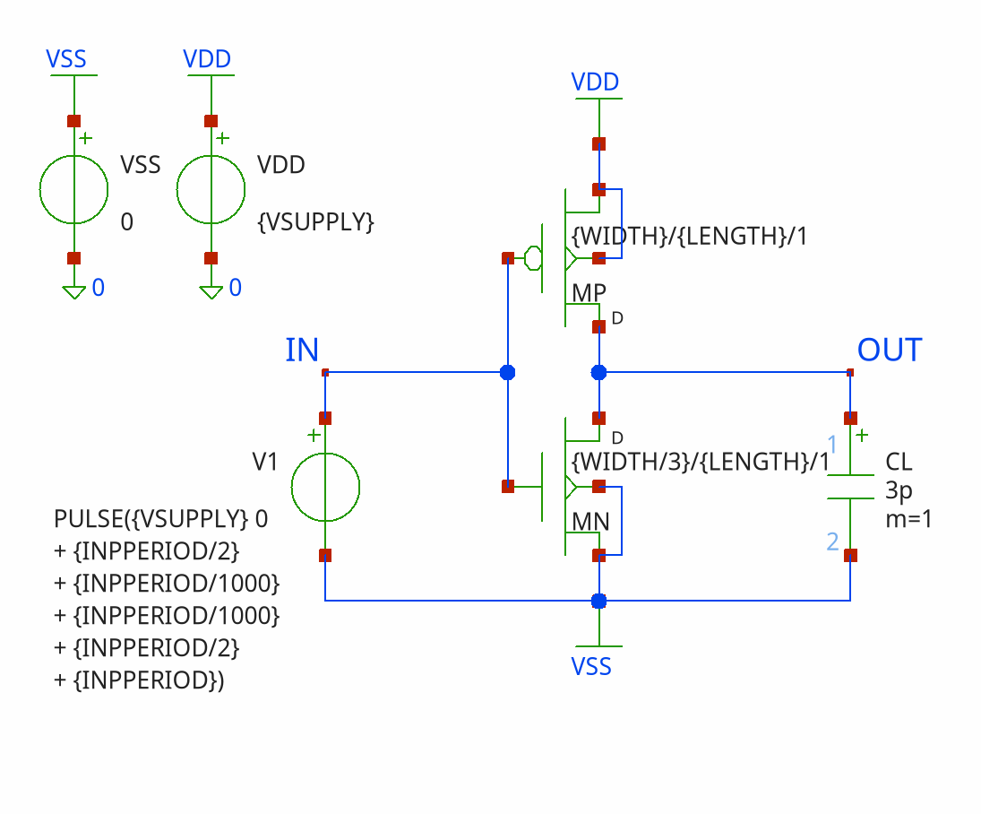
Simulation is done with pulsed input signal 4 periods long. We use three diffrerent supply voltage values to make result be optimal across possible range of power levels. The goal is to find width PWIDTH of PMOS transistor that provide minimum possible power consumption while satisfy certain constraints: low state output voltage value to be no more than certain value VLOWLIM and high state output voltage value to be no less than certain value VHIGHLIM.
Input parameters and constraints values are:
| 2V, 2.1V, 2.2V. | |
| 0.05V. | |
| 1.95V. | |
| 850MHz. | |
| 0.35um. | |
| 4. |
Width NWIDTH of NMOS device is 3 times lower than width PWIDTH of PMOS device. Lengths of bothe devices are equal to LENGTH. Perimeters of source and drain for both devices are defined by the equation:
PD = PS = 2 ⋅ (WIDTH + LENGTH)
Input period is:
               1
INPPERIOD = ───────
            INPFREQ
The power consumption is defined as RMS value of instant power I(VDD)*V(VDD,VSS) across fourth period time interval defined by TMEASSTART and TMEASSTOP:
TMEASSTART = (NOPERIODS - 1) ⋅ INPPERIOD
TMEASSTOP = NOPERIODS ⋅ INPPERIOD
            ________________________________________________________________
           ╱                          TMEASSTOP
          ╱            1                  ⌠                           2
PRMS =   ╱  ────────────────────── ⋅      ⌡     (I(VDD) ⋅ V(VDD, VSS))  ⋅ dt
       ╲╱   TMEASSTOP - TMEASSTART   TMEASSTART
Low and high voltages values are measured at fourth output pulse at times TMEAS1 and TMEAS2 correspondingly:
                     3.0 ⋅ INPPERIOD
TMEAS1 = TMEASSTOP - ───────────────
                           4.0
                     INPPERIOD
TMEAS2 = TMEASSTOP - ─────────
                        4.0
In the next code lines we define all above mentioned constants as well as equations for PD and PS:
proc pdPsCalc {width length} {
    return [= {2*$width+2*$length}]
}
# set parameters
set vSupply 2.0
set inpFreq 850e6
set inpPeriod [= {1.0/$inpFreq}]
set noPeriods 4
set tmeasStart [= {($noPeriods-1)*$inpPeriod}]
set tmeasStop [= {$noPeriods*$inpPeriod}]
set tmeas1 [= {$tmeasStop-3.0*$inpPeriod/4.0}]
set tmeas2 [= {$tmeasStop-1.0*$inpPeriod/4.0}]
set initialPWidth 10e-3
set pWidth $initialPWidth
set nWidth [= {$pWidth/3.0}]
set length 0.35e-6
set vLowLim 0.05
set vHighLim 1.95
set pd [pdPsCalc $pWidth $length]
set ps [pdPsCalc $pWidth $length]
set vSupplyVals {2.0 2.1 2.2}
Next step is to define circuit with all mentioned values calculated previously, and add .include statement for NMOS and PMOS models with class ::SpiceGenTcl::Include:
# build circuit
set circuit [Circuit new {Inverter}]
set vdd [Vdc new dd vdd 0 -dc $vSupply]
set vss [Vdc new ss vss 0 -dc 0.0]
set vIn [Vpulse new 1 in vss -low $vSupply -high 0.0 -td [= {$inpPeriod/2.0}] -tr [= {$inpPeriod/1000.0}] -tf [= {$inpPeriod/1000.0}] -pw [= {$inpPeriod/2.0}] -per $inpPeriod]
set capLoad [C new l out vss -c 3p]
set mp [M new p out in vdd -model pmos -l $length -w $pWidth -n4 vdd -pd $pd -ps $ps]
set mn [M new n out in vss -model nmos -l $length -w $nWidth -n4 vss -pd $pd -ps $ps]
$circuit add $vdd $vss $vIn $capLoad $mp $mn
$circuit add [Tran new -tstep [= {$inpPeriod/1000.0}] -tstop [= {$inpPeriod*$noPeriods}]]
$circuit add [Include new [file join $scriptPath models n.typ]]
$circuit add [Include new [file join $scriptPath models p.typ]]
Also we define simulator (Ngspice) that should be used:
# set simulator
if {[catch {set simulator [Shared new batch1]}]} {
    set simulator [Batch new batch1]
}
$circuit configure -simulator $simulator
It is better to use ::SpiceGenTcl::Ngspice::Simulators::Shared because of speed improvement - we read data right from the memory and skipping phase of reading saving and reading raw file. But for that we need to have companion package NgspiceTclBridge and compiled shared Ngspice for your platform. If it is not done, we fallback to usual ::SpiceGenTcl::Ngspice::Simulators::Batch version.
Next large step is to define correct cost function that taking into account the constraints voltages VLOWLIM and VHIGHLIM, the power consumption PRMS and different values of VSUPPLY voltages.
The general equation for cost function is:
              i = n                    ⎛P      - P    ⎞
              ____                     ⎜ spec     sim ⎟
              ╲                        ⎜     j       j⎟
Cost = W    ⋅  ╲    P     + W    ⋅ max ⎜──────────────⎟
        obj    ╱     sim     con       ⎜    P         ⎟
              ╱         i              ⎜     spec     ⎟
              ‾‾‾‾                     ⎝         j    ⎠
              i = 1                                    j∈[1,m]
where:
P_sim_i- performance metrics (objectives), in our case it is power consumptionPMRS, so n=1.W_obj- weight for each objectives.P_spec_jandP_sim_j- constraints metrics, specified and simulated respectively. In out case these constraints are voltagesVHIGHLIMandVLOWLIM, so m=2. In cost function we include only the maximum relative error from all constraints.W_con- weight for contraints.
In our case we use three supply voltages VSUPPLY, so cost function is calculated for each one and summed.
The tricky part is to select right weights for both objectives and constraints. When we are satisfied constraints, the value should be neglegible to objective member value, but when we are do not satisfy the constraints, we should get large increase in overall cost function so we avoid going beyond these constraints. Sometimes correction is necessary in case optimization does not gradually improving, or we ended up with violated constraints.
In our case we have constraints:
- Low voltage must be equal or lower than
VLOWLIM, so cost error function should increase if low voltage is higher, and be small or zero if we are below the limit. - High voltage must be equal or higher than
VHIGHLIM, so cost function should increase if high voltage is lower, and be small or zero if we are below the limit.
By default the W_obj is set to 10, so W_con should be in between 100-10000, and it's better to start from the higher value, so we set it to 10000.
So, the final cost function is:
set pdata [dcreate vSupplyVals $vSupplyVals nDevice $mn pDevice $mp vLowLim $vLowLim vHighLim $vLowLim length $length vdd $vdd tmeas1 $tmeas1 tmeas2 $tmeas2 objWeight 10 constrWeight 10000 circuit $circuit]
proc costFunc {xall pdata args} {
    dict with pdata {}
    set width [@ $xall 0]
    set pdPs [pdPsCalc $width $length]
    $nDevice actOnParam -set l $length w [= {$width/3.0}] pd $pdPs ps $pdPs
    $pDevice actOnParam -set l $length w $width pd $pdPs ps $pdPs
    foreach val $vSupplyVals {
        $vdd actOnParam -set dc $val
        if {[catch {$circuit runAndRead}]} {
            # huge penalty in case of non-convergence
            lappend vlowList 1
            lappend vhighList 1
            lappend psupplyList 1
            continue
        }
        set data [$circuit getDataDict]
        lappend vlowList [measure -xname time -data $data -find v(out) -at $tmeas1]
        lappend vhighList [measure -xname time -data $data -find v(out) -at $tmeas2]
        set instantPower [= {mul([dget $data i(vdd)], [dget $data v(vdd)])}]
        lappend psupplyList [measure -xname time -data [dcreate time [dget $data time] instantPower $instantPower] -rms "-vec instantPower -from $tmeas1 -to $tmeas2"]
    }
    set costObj 0.0
    set costConstr 0.0
    foreach psupply $psupplyList vlow $vlowList vhigh $vhighList {
        set constrVlow [= {($vlow-$vLowLim)/$vLowLim}]
        if {$constrVlow<0} {
            set constrVlow 0.0
        }
        set constrVhigh [= {($vHighLim-$vhigh)/$vHighLim}]
        if {$constrVhigh<0} {
            set constrVhigh 0.0
        }
        set costObj [= {$costObj+$psupply}]
        set costConstr [= {$costConstr+max($constrVlow, $constrVhigh)}]
    }
    return [= {$objWeight*$costObj+$constrWeight*$costConstr}]
}
Let's breakdown it line by line to clarify every step while keeping in mind the previous information.
First, we build pdata dictionary with information that is necessary to evaluate the cost function:
set pdata [dcreate vSupplyVals $vSupplyVals nDevice $mn pDevice $mp vLowLim $vLowLim vHighLim $vLowLim length $length vdd $vdd tmeas1 $tmeas1 tmeas2 $tmeas2 objWeight 10 constrWeight 10000 circuit $circuit]
vSupplyVals- list of power supply voltagesnDevice- NMOS transistor object from the circuit we built, used to change parameters of the devicepDevice- NMOS transistor object from the circuit we built, used to change parameters of the devicevLowLim- value of lower limit constraintVLOWLIMvHighLim- value of lower limit constraintVHIGHLIMlength- length of both NMOS and PMOS transistorsvdd- power source object from the circuit we built, used to change parameters of the devicetmeas1- start of the power measure intervaltmeas2- end of the power measure intervalobjWeight- objective weight valueconstrWeight- constraints weight valuecircuit- circuit object we use to produce netlist
At the start we unpack the dictionary to local variables with the same name as key of the dictionary. Then we extract the WIDTH parameter from vectors of variables. We have only one variable, so we just get first and the only element:
dict with pdata {}
set width [@ $xall 0]
Next we calculate the pd and ps parameters from the given length and and new width, and change the parameters of NMOS and PMOS devices with the new values:
set pdPs [pdPsCalc $width $length]
$nDevice actOnParam -set l $length w [= {$width/3.0}] pd $pdPs ps $pdPs
$pDevice actOnParam -set l $length w $width pd $pdPs ps $pdPs
In the next block we loop over all power supply voltages, run circuit, read the data and extract values we need:
foreach val $vSupplyVals {
    $vdd actOnParam -set dc $val
    if {[catch {$circuit runAndRead}]} {
        # huge penalty in case of non-convergence
        lappend vlowList 1
        lappend vhighList 1
        lappend psupplyList 1
        continue
    }
    set data [$circuit configure -data]
    set dataDict [$circuit getDataDict]
    lappend vlowList [$data measure -find v(out) -at $tmeas1]
    lappend vhighList [$data measure -find v(out) -at $tmeas2]
    set instantPower [= {mul([dget $dataDict i(vdd)], [dget $dataDict v(vdd)])}]
    lappend psupplyList [measure -xname time -data [dcreate time [dget $dataDict time] instantPower $instantPower] -rms "-vec instantPower -from $tmeas1 -to $tmeas2"]
}
An additional guard was added to prevent stepping into regions where circuit could fail due to non-convergence, so we set objective and constraints metric to high values:
if {[catch {$circuit runAndRead}]} {
    # huge penalty in case of non-convergence
    lappend vlowList 1
    lappend vhighList 1
    lappend psupplyList 1
    continue
}
To find values VLOW and VHIGH we use method ::SpiceGenTcl::RawFile::measure, that is wrapper to measure command from package tclmeasure. Then we calculate calculate instant power by multiplying current through power source to power voltage, and then directly use command measure from package tclmeasure:
set data [$circuit configure -data]
set dataDict [$circuit getDataDict]
lappend vlowList [$data measure -find v(out) -at $tmeas1]
lappend vhighList [$data measure -find v(out) -at $tmeas2]
set instantPower [= {mul([dget $dataDict i(vdd)], [dget $dataDict v(vdd)])}]
lappend psupplyList [measure -xname time -data [dcreate time [dget $dataDict time] instantPower $instantPower] -rms "-vec instantPower -from $tmeas1 -to $tmeas2"]
After looping through all power voltages, we get values of objective in list psupplyList and constraints for VLOW and VHIGH in lists vlowList and vhighList correspondingly.
In the final block we calculate value of cost function according to equations provided previously:
set costObj 0.0
set costConstr 0.0
foreach psupply $psupplyList vlow $vlowList vhigh $vhighList {
    set constrVlow [= {($vlow-$vLowLim)/$vLowLim}]
    if {$constrVlow<0} {
        set constrVlow 0.0
    }
    set constrVhigh [= {($vHighLim-$vhigh)/$vHighLim}]
    if {$constrVhigh<0} {
        set constrVhigh 0.0
    }
    set costObj [= {$costObj+$psupply}]
    set costConstr [= {$costConstr+max($constrVlow, $constrVhigh)}]
}
return [= {$objWeight*$costObj+$constrWeight*$costConstr}]
After defining cost function, we can initialize and run optimization. As optimization engine we use Differential Evolution algorithm from tclopt packkage:
set par [::tclopt::Parameter new width $pWidth -lowlim 1e-4 -uplim 10e-3]
set optimizer [::tclopt::DE new -funct costFunc -pdata $pdata -strategy rand-to-best/1/exp -genmax 50 -refresh 1 -np 10 -f 0.5 -cr 1 -seed 3 -debug -abstol 1e-6 -history -histfreq 1]
$optimizer addPars $par
set width [dget [$optimizer run] x]
In first line we create parameter object and set the boundaries for the width value, from 100um to 10mm. Strategy selection, values of f, cr, np and genmax are the same as in ASCO example. Then we add parameter object par to optimizer object optimizer, run it, and wait for the result. We set debug mode with -debug switch to see progress output, and also we save history to look at the best trajectory of optimum searching.
In the next block we read history information that is saved during the optimization, it was turned on by -history switch:
# get results and history
set results [$optimizer run]
set width [dget $results x]
set trajectory [dict get $results besttraj]
set bestf [dict get $results history]
foreach genTr $trajectory genF $bestf {
    lappend optData [list {*}[dict get $genTr x] [dict get $genF bestf]]
    lappend functionTrajectory [list [dict get $genTr gen] [dict get $genTr x]]
}
The we plot trajectory with ticklecharts package:
# plot 2D trajectory
set chart [ticklecharts::chart new]
$chart Xaxis -name "Generation" -minorTick {show "True"} -type "value" -splitLine {show "True"}
$chart Yaxis -name "Cost function" -minorTick {show "True"}  -splitLine {show "True"}
$chart SetOptions -title {} -tooltip {trigger "axis"} -animation "False" -toolbox {feature {dataZoom {yAxisIndex "none"}}}
$chart Add "lineSeries" -name "Best trajectory" -data $functionTrajectory -showAllSymbol "nothing"
set fbasename [file rootname [file tail [info script]]]
$chart Render -outfile [file normalize [file join .. html_charts ${fbasename}_plot.html]]
The final block of code is for calculating initial and final values of VLOW, VHIGH, VSUPPLY and preparing waveform for plotting. We calculate it only for highest supply voltage to avoid cluttering:
# calculate initial waveforms the highest supply voltage
set pdPs [pdPsCalc $initialPWidth $length]
$mn actOnParam -set l $length w [= {$initialPWidth/3.0}] pd $pdPs ps $pdPs
$mp actOnParam -set l $length w $initialPWidth pd $pdPs ps $pdPs
$vdd actOnParam -set dc [@ $vSupplyVals 2]
$circuit runAndRead
set data [$circuit configure -data]
set dataDict [$circuit getDataDict]
foreach timeVal [dget $dataDict time] voutVal [dget $dataDict v(out)] {
    lappend initialWaveform [list $timeVal $voutVal]
}
set vlowInitial [$data measure -find v(out) -at $tmeas1]
set vhighInitial [$data measure -find v(out) -at $tmeas2]
set instantPower [= {mul([dget $dataDict i(vdd)], [dget $dataDict v(vdd)])}]
set psupplyInitial [measure -xname time -data [dcreate time [dget $dataDict time] instantPower $instantPower] -rms "-vec instantPower -from $tmeas1 -to $tmeas2"]

# calculate final waveform for the highest supply voltage
set pdPs [pdPsCalc $width $length]
$mn actOnParam -set l $length w [= {$width/3.0}] pd $pdPs ps $pdPs
$mp actOnParam -set l $length w $width pd $pdPs ps $pdPs
$vdd actOnParam -set dc [@ $vSupplyVals 2]
$circuit runAndRead
set data [$circuit configure -data]
set dataDict [$circuit getDataDict]
foreach timeVal [dget $dataDict time] voutVal [dget $dataDict v(out)] {
    lappend finalWaveform [list $timeVal $voutVal]
}
set vlowFinal [$data measure -find v(out) -at $tmeas1]
set vhighFinal [$data measure -find v(out) -at $tmeas2]
set instantPower [= {mul([dget $dataDict i(vdd)], [dget $dataDict v(vdd)])}]
set psupplyFinal [measure -xname time -data [dcreate time [dget $dataDict time] instantPower $instantPower] -rms "-vec instantPower -from $tmeas1 -to $tmeas2"]
Plotting initial and final waveforms, and result values:
# plot waveforms
set chart [ticklecharts::chart new]
$chart Xaxis -name "Time, s" -minorTick {show "True"} -type "value" -splitLine {show "True"}
$chart Yaxis -name "v(out)" -minorTick {show "True"}  -splitLine {show "True"}
$chart SetOptions -title {} -legend {} -tooltip {trigger "axis"} -animation "False" -toolbox {feature {dataZoom {yAxisIndex "none"}}}
$chart Add "lineSeries" -name "initial, vdd=[@ $vSupplyVals 2]" -data $initialWaveform -showAllSymbol "nothing" -symbolSize "0"
$chart Add "lineSeries" -name "final, vdd=[@ $vSupplyVals 2]" -data $finalWaveform -showAllSymbol "nothing" -symbolSize "0"

set fbasename [file rootname [file tail [info script]]]
$chart Render -outfile [file normalize [file join .. html_charts ${fbasename}_waveforms_plot.html]]

# print resulted values for the highest supply voltage
puts "Optimization succesfully finished at generation [dget $results generation], total number of function evaluations - [dget $results nfev]"
puts "Convergence info: [dget $results info]"
puts "Best value of cost function is [format "%3e" [dget $results objfunc]]"
puts "Final width of PMOS is [format "%.3f" [= {$width/1e-3}]]mm, from initial value [format "%.3f" [= {$initialPWidth/1e-3}]]mm"
puts "For VDD=[@ $vSupplyVals 2]V, VLOW: [format "%.3f" $vlowInitial]V → [format "%.3f" $vlowFinal]V<[format "%.3f" $vLowLim]V, VHIGH: [format "%.3f" $vhighInitial]V → [format "%.3f" $vhighFinal]V>[format "%.3f" $vHighLim]V, PSUPPLY: [format "%.3f" $psupplyInitial]W → [format "%.3f" $psupplyFinal]W"
Waveforms are:
And final numbers:
Optimization succesfully finished at generation 12, total number of function evaluations - 130
Convergence info: Optimization stopped due to crossing threshold 'abstol+reltol*abs(mean)=0.030176353097193406' of objective function population member standard deviation
Best value of cost function is 2.984087e+00
Final width of PMOS is 0.789mm, from initial value 10.000mm
For VDD=2.2V, VLOW: 0.147V → 0.046V<0.050V, VHIGH: 2.020V → 2.161V>1.950V, PSUPPLY: 1.101W → 0.107W