Tutorials

Tutorials in this section describes examples from folder examples in root directory of SpiceGenTcl. List of availible tutorials:

• Netlist manipulations - “examples/netlist_manipulations.tcl” file

• Subcircuit definition - “examples/subcircuit.tcl” file

• Diode current simualtion - “examples/ngspice/dc/diode_iv.tcl”, “examples/xyce/dc/diode_iv.tcl” and “examples/ltspice/dc/diode_iv.tcl” files.

• Diode capacitance simualtion - “examples/ngspice/ac/diode_cv.tcl”, “examples/xyce/ac/diode_cv.tcl” and “examples/ltspice/ac/diode_cv.tcl” files.

• Sensitive analysis of differential pair - “examples/ngspice/sens/diffpair_sens.tcl” file

• Transient simulation of ring oscillator - “examples/ngspice/transient/switch_oscillator.tcl”, “examples/xyce/transient/switch_oscillator.tcl” and “examples/ltspice/transient/switch_oscillator.tcl” files.

• Transient simulation of four-bit adder - “examples/ngspice/transient/fourbitadder.tcl”, “examples/xyce/transient/fourbitadder.tcl” “examples/ltspice/transient/fourbitadder.tcl” files

• S-parameter simulation of pass-band filter - “examples/ngspice/sp/filter.tcl”

Netlist manipulations

In this example we will examine the availible actions that we can do on elements in netlist. First step is building the target netlist with variable elements:

set netlist [Netlist new main_netlist]

# incrementally build netlist by adding different elements
$netlist add [R new 1 net1 net2 -r 10]
$netlist add [R new 5 net1 net2 -model res_sem -l 10e-6 -w 100e-6]
$netlist add [RModel new rsem1mod -tc1 0.1 -tc2 0.4]
$netlist add [R new 2 net1 net2 -r {-eq {r1+5/10}}]
$netlist add [C new 1 net2 net3 -c 1e-6]
$netlist add [ParamStatement new {{r1 1} {r2 2}} -name ps1]
$netlist add [Comment new {some random comment} -name com1]
$netlist add [Include new {/fold1/fold2/file.lib} -name inc1]
$netlist add [Library new {/fold1/fold2/file.lib} fast -name lib1]
$netlist add [RawString new {*comment in form of raw string} -name raw1]
$netlist add [Vdc new 1 net1 net3 -dc 5]
$netlist add [Tran new -tstep 1e-6 -tstop 1e-3 -uic -name tran1]

Here we can see the ::SpiceGenTcl::Netlist::add method that adds elemements objects references to ::SpiceGenTcl::Netlist object. To view netlist we can invoke method ::SpiceGenTcl::Netlist::genSPICEString that have all circuit elements:

puts [$netlist genSPICEString]

Result is:

r1 net1 net2 10
r5 net1 net2 res_sem l=10e-6 w=100e-6
.model rsem1mod r(tc1=0.1 tc2=0.4)
r2 net1 net2 {r1+5/10}
c1 net2 net3 1e-6
.param r1=1 r2=2
*some random comment
.include /fold1/fold2/file.lib
.lib /fold1/fold2/file.lib fast
*comment in form of raw string
v1 net1 net3 5
.tran 1e-6 1e-3 uic

Delete element

The opposite action is to delete with the ::SpiceGenTcl::Netlist::del method. For example, we can delete the ‘c1’ element from the netlist by specifying its name:

$netlist del c1
puts [$netlist genSPICEString]

Result is:

r1 net1 net2 10
r5 net1 net2 res_sem l=10e-6 w=100e-6
.model rsem1mod r(tc1=0.1 tc2=0.4)
r2 net1 net2 {r1+5/10}
.param r1=1 r2=2
*some random comment
.include /fold1/fold2/file.lib
.lib /fold1/fold2/file.lib fast
*comment in form of raw string
v1 net1 net3 5
.tran 1e-6 1e-3 uic

As you can see, capacitor ‘c1’ is no more in netlist.

Get element

Next important operation is getting reference of element in netlist. We can do it again by specifying its name:

set resistor [$netlist getElement r1]

After it, we can change the resistance parameter of element:

$resistor actOnParam -set r 100

We apply method ::SpiceGenTcl::Device::actOnParam with three arguments: -set option that selects action, name of parameter ‘r’ and its new value ‘100’. The other action we can do is change the pin connection of element:

$resistor actOnPin -set np net10

We use method ::SpiceGenTcl::Device::actOnPin with -set option that selects action, pin name and name of the net as arguments.

Then we can again print netlist and see that value of parameter and name of connected name have been changed:

r1 net10 net2 100
r5 net1 net2 res_sem l=10e-6 w=100e-6
.model rsem1mod r(tc1=0.1 tc2=0.4)
r2 net1 net2 {r1+5/10}
.param r1=1 r2=2
*some random comment
.include /fold1/fold2/file.lib
.lib /fold1/fold2/file.lib fast
*comment in form of raw string
v1 net1 net3 5
.tran 1e-6 1e-3 uic

Print list of all elements

We can get the list of all elements attached to $netlist object:

# get and print all names of elements attached to $netlist
puts [$netlist getAllElemNames]

Result:

r1 r5 rsem1mod r2 ps1 com1 inc1 lib1 raw1 v1 tran1

Temporarly remove of element

We can delete element from netlist and store reference to elements object, and then again add element to netlist:

set r1 [$netlist getElement r1]
$netlist del r1
$netlist add $r1

Also, we can save reference to object before adding to netlist in variable and only then add it to netlist:

set r5 [R new 5 net1 net2 -r 10]
$netlist add $r5

In this case we can directly modify ‘r5’ parameters without necessity to call ::SpiceGenTcl::Netlist::getElement method.

Subcircuit definition

To create subcircuit definition we use special ::SpiceGenTcl::Subcircuit class and make subcircuit by defining new class with it as superclass:

oo::class create RCnet {
    superclass Subcircuit
    constructor {} {
        # define external pins of subcircuit
        set pins {plus minus}
        # define input parameters of subcircuit
        set params {{r 100} {c 1e-6}}
        # add elements to subcircuit definition
        my add [R new 1 net1 plus -r {-eq r}]
        my add [C new 1 net2 net3 -c {-eq c}]
        my add [R new 5 minus net2 -model res_sem -l 10e-6 -w 100e-6]
        my add [RModel new rsem1mod -tc1 0.1 -tc2 0.4]
        # pass name, list of pins and list of parameters to Subcircuit constructor
        next rcnet $pins $params
    }
}

In constructor of this class we define pins as list with names in order of appearance in subcircuit header:

set pins {plus minus}

Then we define parameters as list of two-elements list that contains name and default value of parameter:

set params {{r 100} {c 1e-6}}

Next step is adding elements to subcircuit:

my add [R new 1 net1 plus -r {-eq r}]
my add [C new 1 net2 net3 -c {-eq c}]
my add [R new 5 minus net2 -model res_sem -l 10e-6 -w 100e-6]
my add [RModel new rsem1mod -tc1 0.1 -tc2 0.4]

The last action is to pass name of subcircuit, list of pins and parameters to constructor of superclass:

next rcnet $pins $params

Name passed to superclass constructor rcnet is not necessarily the same as name of the class, this name will be printed in subcircuit definition in netlist.

To create and add this definition to netlist, we use name of the class RCnet:

# create subcircuit definition
set subcircuit [RCnet new]
# add to netslit
$netlist add $subcircuit

But place definition of subcircuit is not enough - we need to place netlist instance of subcircuit. We can do it by using two mechanisms:

• use ::SpiceGenTcl::Ngspice::BasicDevices::SubcircuitInstance class

• use ::SpiceGenTcl::Ngspice::BasicDevices::SubcircuitInstanceAuto class

First way is direct construction of element by providing pins and parameter lists:

set subInst [SubcircuitInstance new 1 {{plus net1} {minus net2}} rcnet {{r 1} {-eq c cpar}}]

But the second way is simpler and allow to check if we have mistake in definition:

set subInst1 [SubcircuitInstanceAuto new $subcircuit 2 {net1 net2} -r 1 -c {-eq cpar}]

In this approach, we pass the reference of our subcircuit as the first argument. Then, we only need to provide a list of nets connected to the pins, in the order defined in the subcircuit, and parameters in the form of -paramName paramValue. If you try to add a parameter that does not exist in the subcircuit definition, you’ll receive an error.

The final circuit is:

.subckt rcnet plus minus r=100 c=1e-6
r1 net1 plus {r}
c1 net2 net3 {c}
r5 minus net2 res_sem l=10e-6 w=100e-6
.model rsem1mod r(tc1=0.1 tc2=0.4)
.ends rcnet
x1 net1 net2 rcnet r=1 c={cpar}
x2 net1 net2 rcnet r=1 c={cpar}

Diode current simualtion

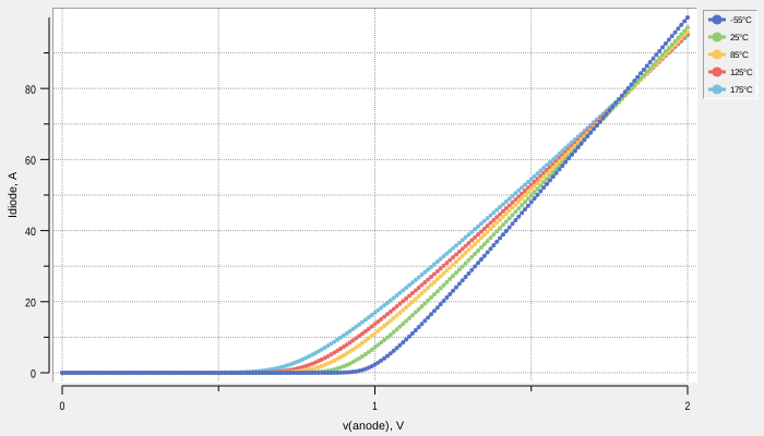
In this example, we examine the parametric simulation of a diode model’s current curve, with the ambient temperature as the parameter. To achieve this, we need to run the simulation multiple times at different temperatures, save the results from each iteration, and then combine them into a single plot.

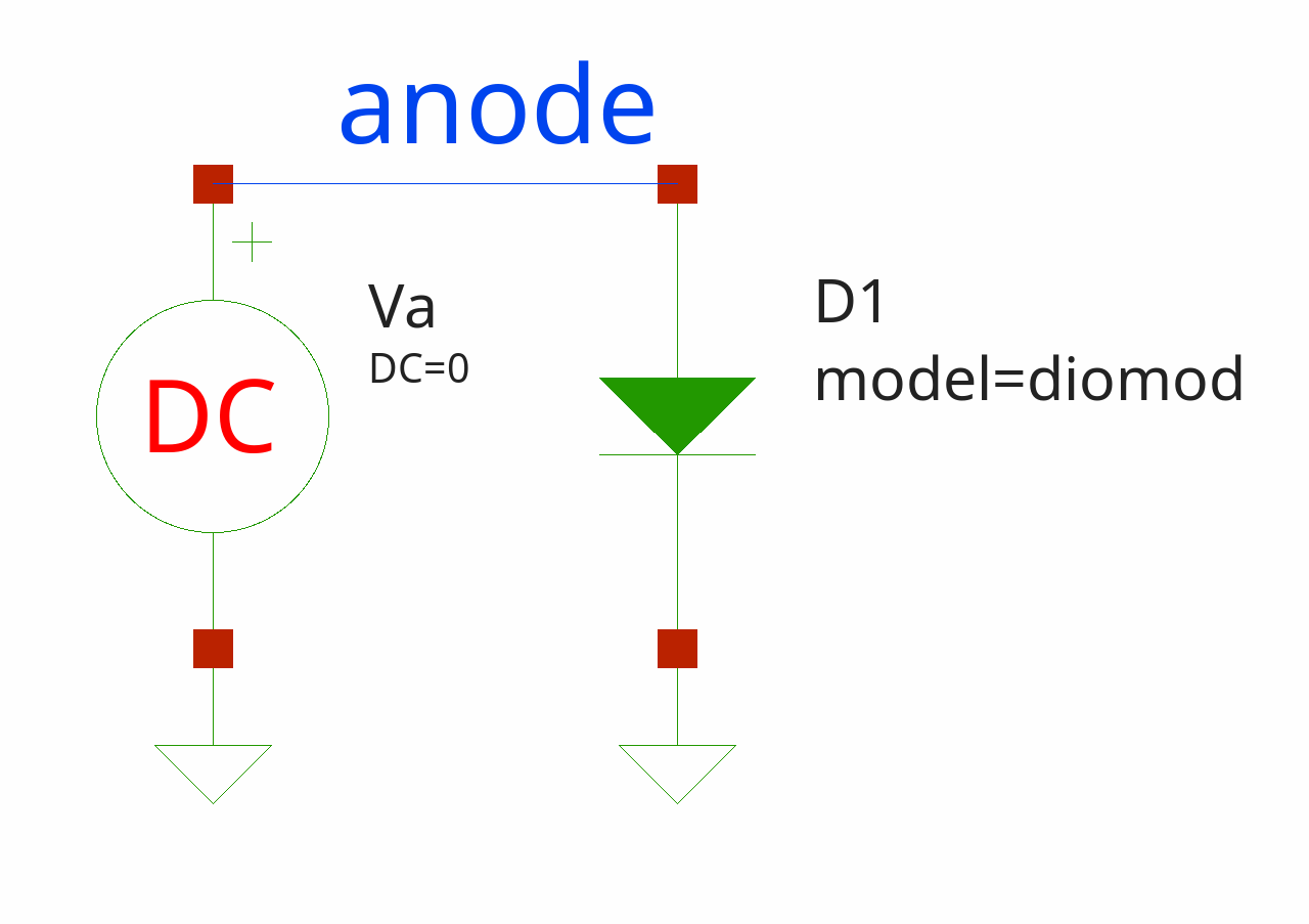
The circuit is simple:

As in previous examples, we start by creating the top circuit and adding elements to it:

set circuit [Circuit new {diode IV}]
# add elements to circuit
$circuit add [D new 1 anode 0 -model diomod -area 1 -lm 1e-6]
$circuit add [Vdc new a anode 0 -dc 0]
$circuit add [DiodeModel new diomod -is 1e-12 -n 1.2 -rs 0.01 -cjo 1e-9 -trs1 0.001 -xti 5 -ikf 100]
$circuit add [Dc new -src va -start 0 -stop 2 -incr 0.01]

In the upper block of code, we add a diode instance using the ::SpiceGenTcl::Ngspice::SemiconductorDevices::D command, create the corresponding diode model with the ::SpiceGenTcl::Ngspice::SemiconductorDevices::DiodeModel command, add a DC voltage source that will be swept, and include a DC analysis statement. The voltage ranges from 0 to 2 volts to obtain the forward current characteristic.

The temperature in Ngspice is set using the .temp statement. We create an instance with the ::SpiceGenTcl::Temp command, save the object reference in the variable tempSt, and then add it to the circuit:

set tempSt [Temp new 25]
$circuit add $tempSt

Next, we create an array containing the temperature values and instantiate an object of the ::SpiceGenTcl::Ngspice::Simulators::Batch class:

# add temperature sweep
set temps {-55 25 85 125 175}

### set simulator with default
if {[catch {set simulator [Shared new -nocleanup shared1]}]} {
    set simulator [Batch new -nocleanup batch1]
}
# attach simulator object to circuit
$circuit configure -simulator $simulator

The only thing left is to set the temperature value in the ::SpiceGenTcl::Temp class object, run the circuit, save the data, and repeat this process multiple times:

foreach temp $temps {
    $tempSt configure -value $temp
    $circuit runAndRead -vector
    set data [$circuit getDataDict]
    lappend xVecs [dict get $data v(anode)]
    set yVec [dict get $data i(va)]
    $yVec expr {-$yVec}
    lappend yVecs $yVec
}

Plotting the results:

set chart [ticklecharts::chart new]
set numberFormat [ticklecharts::jsfunc new {
    function (value) {
        return Number(value).toPrecision(4);
    }
}]
$chart Xaxis -name {v(anode), V} -minorTick {show True} -type value -splitLine {show True}
$chart Yaxis -name {Idiode, A} -minorTick {show True} -type value -splitLine {show True}
$chart SetOptions -title {} -tooltip [list trigger axis valueFormatter $numberFormat] -animation False -legend {}\
        -toolbox {feature {dataZoom {yAxisIndex none}}} -grid {left 5% right 15%}
foreach xVec $xVecs yVec $yVecs temp $temps {
    $chart Add lineSeries -data [transpose [list [$xVec index :] [$yVec index :]]] -showAllSymbol nothing\
            -name ${temp}°C -symbolSize 2
}
set fbasename [file rootname [file tail [info script]]]
$chart Render -outfile [file normalize [file join .. html_charts $fbasename.html]] -width 800px -height 500px\
        -divid $fbasename -jschartvar chart_$fbasename -jsvar option_$fbasename

In the picture, you can see how temperature affects the forward current of the diode. Because the series resistance has a temperature dependence, all the lines intersect near 1.8V, indicating the point of zero temperature coefficient.

If rbc package is installed, plotting could be done with it:

if {![catch {package require rbc::graphtoolbar}]} {
    set colors {#5470c6 #91cc75 #fac858 #ee6666 #73c0de #3ba272 #fc8452 #9a60b4 #ea7ccc}
    set graph [rbc::graphtoolbar .g -width 700 -height 400 -type graph -controlmode context -zoom -crosshairs\
                       -crosshairsmode closest -crosshairsclosestopts {-interpolate no} -pan -zoomwheel -scaletoggle y\
                       -activelegend]
    $graph graph grid on
    $graph graph axis configure x -title {v(anode), V}
    $graph graph axis configure y -title {Idiode, A}
    set i -1
    foreach xVec $xVecs yVec $yVecs temp $temps {
        $graph graph element create temp$temp -x $xVec -y $yVec -symbol circle -pixels 2 -label ${temp}°C\
                -color [lindex $colors [incr i]]
    }
    grid $graph -sticky nsew
    grid columnconfigure . 0 -weight 1
    grid rowconfigure . 0 -weight 1
    $graph graph svg output [file normalize [file join .. .. .. docs assets img svg_charts ngspice $fbasename.svg]]
}

This circuit works without modification in LTspice simulator, see “examples/ltspice/dc/diode_iv.tcl” file.

For Xyce simulator there are some differences, see “examples/xyce/dc/diode_iv.tcl” file. The one of the differences is how we set the global temperature: in Xyce there is no .temp statement, for setting global temperature we use .options statement with class ::SpiceGenTcl::Options:

set tempSt [Options new {{-sw device} {temp 25}}]

and then modify this value in loop:

$tempSt actOnParam -set temp $temp

Also, the names of the resulted vectors are different:

lappend xVecs [dict get $data anode]
set yVec [dict get $data va#branch]

Diode capacitance simualtion

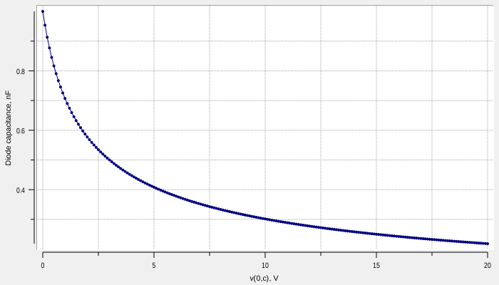
In this example, we measure the volt-farad (or capacitance-voltage) relationship of the diode’s depletion charge. To achieve this, we need to apply a negative voltage bias to the anode and perform an AC simulation at a single frequency. We then repeat this process at different voltages, collect all the results, and finally plot the entire curve. We calculate the capacitance value using the following equation:

          ⎛I⎞
      -Im ⎜─⎟
          ⎝V⎠
C = ────────────
    2 ⋅ π ⋅ freq

where I and V - voltage and current phasors, freq - frequency of applied AC signal. First, we can define π constant manually, or borrow the value from ::math::constants library:

package require math::constants
::math::constants::constants radtodeg degtorad pi
variable pi

We again go through the circuit building sequence:

set circuit [Circuit new {diode CV}]
# add elements to circuit
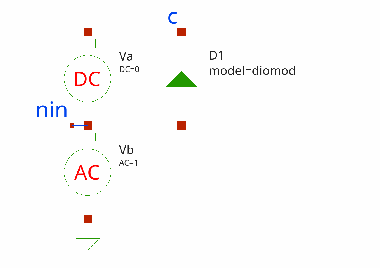
$circuit add [D new 1 0 c -model diomod -area 1 -lm 1e-6]
set vdc [Vdc new a c nin -dc 0]
$circuit add $vdc
$circuit add [Vac new b nin 0 -ac 1]
$circuit add [DiodeModel new diomod -is 1e-12 -n 1.2 -rs 0.01 -cjo 1e-9 -trs1 0.001 -xti 5]
$circuit add [Ac new -name ac -variation lin -n 1 -fstart 1e5 -fstop 1e5]

What is new here:

• AC voltage source [Vac new b nin 0 -ac 1] - uses to generate AC signal

• AC analysis statement [Ac new -variation lin -n 1 -fstart 1e5 -fstop 1e5] - uses to define AC frequency, 100 kHz in our case.

The final circuit looks like this:

Nest step is to add voltage sweep:

set voltSweep [lseq 0 20.0 0.1]

Then we as usual, create ::SpiceGenTcl::Ngspice::Simulators::Batch (or ::SpiceGenTcl::Ngspice::Simulators::Shared if availible) class object, attach it to $circuit, run it multiple times, collect results and apply the equation to calculate the capacitance (with the voltage phasor set to 1, so it is omitted):

if {[catch {set simulator [Shared new shared1]}]} {
    set simulator [Batch new batch1]
}
# attach simulator object to circuit
$circuit configure -simulator $simulator

### loop in which we run simulation, change reverse bias and read the results
vector create y -type complex
vector create voltage
foreach volt $voltSweep {
    #set reverse voltage bias
    $vdc actOnParam -set dc $volt
    # run simulation
    $circuit runAndRead
    # get data object
    set data [$circuit getDataDict]
    # append data to vectors
    voltage append $volt
    y append [dict get $data i(va)]
}
vector create capacitance
set freq [[$circuit getElement ac] actOnParam -get fstart]
capacitance expr {-imag(y)/(2*$pi*$freq*1e-9)}
set xydata [transpose [list [voltage index :] [capacitance index :]]]

Here, we collect the imaginary component of the current flowing through the AC voltage source ‘Va’.

The AC data vectors are saved into complex RBC vector y.

Now we can plot the results:

set chart [ticklecharts::chart new]
set numberFormat [ticklecharts::jsfunc new {
    function (value) {
        return Number(value).toPrecision(2);
    }
}]
$chart Xaxis -name {v(0,c), V} -minorTick {show True} -type value -splitLine {show True}
$chart Yaxis -name {Diode capacitance, nF} -minorTick {show True} -type value -splitLine {show True}
$chart SetOptions -title {} -tooltip [list trigger axis valueFormatter $numberFormat] -animation False\
        -toolbox {feature {dataZoom {yAxisIndex none}}}
$chart Add lineSeries -name Capacitance -data $xydata -showAllSymbol nothing
set fbasename [file rootname [file tail [info script]]]
$chart Render -outfile [file normalize [file join .. html_charts $fbasename.html]] -width 800px -height 500px\
        -divid $fbasename -jschartvar chart_$fbasename -jsvar option_$fbasename

As a result, we obtain the expected curve, showing a decrease in capacitance value with higher reverse voltage.

If rbc package is installed, plotting could be done with it:

if {![catch {package require rbc::graphtoolbar}]} {
    set graph [rbc::graphtoolbar .g -width 700 -height 400 -type graph -controlmode context -zoom -crosshairs\
                       -crosshairsmode closest -crosshairsclosestopts {-interpolate no} -pan -zoomwheel]
    $graph graph legend configure -hide yes
    $graph graph grid on
    $graph graph axis configure x -title {v(0,c), V}
    $graph graph axis configure y -title {Diode capacitance, nF}
    $graph graph element create current -x voltage -y capacitance -symbol circle -pixels 2
    grid $graph -sticky nsew
    grid columnconfigure . 0 -weight 1
    grid rowconfigure . 0 -weight 1
    $graph graph svg output [file normalize [file join .. .. .. docs assets img svg_charts ngspice $fbasename.svg]]
}

Sensitive analysis of differential pair

In this circuit we run DC sensitive analysis of differential pair.

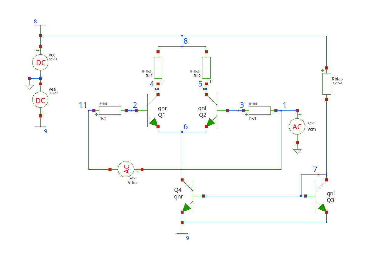
We build circuit step by step:

set circuit [Circuit new {simple differential pair}]
# add elements to circuit
$circuit add [Vdc new cc 8 0 -dc 12] [Vdc new ee 9 0 -dc -12] [Vac new cm 1 0 -ac 1] [Vac new dm 1 11 -ac 1]\
        [Q new 1 4 2 6 -model qnr] [Q new 2 5 3 6 -model qnl] [R new s1 11 2 -r 1e3] [R new s2 3 1 -r 1e3]\
        [R new c1 4 8 -r 10e3] [R new c2 5 8 -r 10e3] [Q new 3 7 7 9 -model qnl] [Q new 4 6 7 9 -model qnr]\
        [R new bias 7 8 -r 20e3]

Then we add models for NPN and PNP bipolar transistors:

$circuit add [BjtGPModel new qnl npn -bf 80 -rb 100 -cjc 2e-12 -tf 0.3e-9 -tr 6e-9 -cje 3e-12 -cjc 2e-12 -vaf 50]
$circuit add [BjtGPModel new qnr npn -bf 80 -rb 100 -cjc 2e-12 -tf 0.3e-9 -tr 6e-9 -cje 3e-12 -cjc 2e-12 -vaf 50]

In DC sensistive analysis we add input voltage to which we sense ohter parameters in the circuit:

$circuit add [SensDc new -outvar v(5,4)]

We create simulator, run it and read data:

set simulator [Batch new {batch1}]
# attach simulator object to circuit
$circuit configure -simulator $simulator
# run circuit, read log and data
$circuit runAndRead
# get data object
set data [$circuit getDataDict]
set vrc1 [dict get $data v(rc1)]
set vrc2 [dict get $data v(rc2)]
puts [format {vrc1=%.3e vrc2=%.3e} $vrc1 $vrc2]

To print resulted sensitivities we use format command where we specify the format of the number:

vrc1=6.032e-04
vrc2=-6.032e-04

Transient simulation of ring oscillator

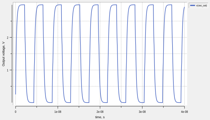
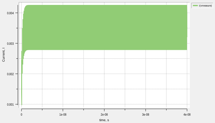
In this example, we analyze a circuit with transient analysis and demonstrate how to use a Tcl script to build a circuit containing multiple stages of the same subcircuit.

The circuit is a ring oscillator composed of voltage-controlled switches, based on an example from Ngspice (/examples/p-to-n-examples/switch-oscillators.cir). Each stage of the oscillator is a simple two-switch inverter, and the entire circuit consists of 17 stages.

At the beginning, we create a class called Inverter to describe the inverter and then instantiate an object of this class:

oo::class create Inverter {
    superclass Subcircuit
    constructor {} {
        # define external pins of subcircuit
        set pins {in out vdd dgnd}
        # define input parameters of subcircuit
        set params {}
        # add elements to subcircuit definition
        my add [C new l out dgnd -c 0.1e-12] [C new 2 out vdd -c 0.1e-12]
        my add [VSwitch new p out vdd vdd in -model swswitch] [VSwitch new n out dgnd in dgnd -model switchn]
        # pass name, list of pins and list of parameters to Subcircuit constructor
        next inverter $pins $params
    }
}

# create subcircuit definition instance
set inverter [Inverter new]

Next, we define the other elements and the top-level circuit:

set circuit [Circuit new {switch_oscillator}]
# add elements to circuit
$circuit add [Tran new -tstep 50e-12 -tstop 40e-9]
$circuit add [Options new {{method gear} {maxord 3}}]
$circuit add [RawString new {.ic v(osc_out)=0.25}]
$circuit add $inverter
$circuit add [Vdc new dd vdd2 0 -dc 3]
$circuit add [Vdc new measure vdd2 vdd -dc 0]
$circuit add [C new vdd vdd 0 -c 1e-18]

We can add multiple stages of inverters using a loop, which saves many lines of code and allows us to dynamically adjust the number of stages:

for {set i 1} {$i<16} {incr i} {
    set ip1 [+ $i 1]
    lappend invsList [SubcircuitInstanceAuto new $inverter x$ip1 "n$i n$ip1 vdd 0"]
}
$circuit add {*}$invsList

After that, we add the first and last stages, as well as the models of the switches:

$circuit add [SubcircuitInstanceAuto new $inverter x18 {osc_out n1 vdd 0}]
$circuit add [SubcircuitInstanceAuto new $inverter x19 {n16 osc_out vdd 0}]
$circuit add [VSwitchModel new swswitch -vt 1 -vh 0.1 -ron 1e3 -roff 1e12]
$circuit add [VSwitchModel new switchn -vt 1 -vh 0.1 -ron 1e3 -roff 1e12]

Now we can run and read data:

if {[catch {set simulator [Shared new shared1]}]} {
    set simulator [Batch new batch1]
}
# attach simulator object to circuit
$circuit configure -simulator $simulator
# run circuit, read log and data
$circuit runAndRead -vector
# get data object
set data [$circuit getDataDict]
set time [dict get $data time]
set vout [dict get $data v(osc_out)]
set imeas [dict get $data i(vmeasure)]
set timeVout [transpose [list [$time index :] [$vout index :]]]
set timeImeas  [transpose [list [$time index :] [$imeas index :]]]

We save output waveform and power currents, and then plot it:

# chart for output voltage
set numberFormat [ticklecharts::jsfunc new {
    function (value) {
        return Number(value).toPrecision(3);
    }
}]
set chartVout [ticklecharts::chart new]
$chartVout Xaxis -name {time, s} -minorTick {show True} -type value -splitLine {show True}
$chartVout Yaxis -name {Output voltage, V} -minorTick {show True} -type value -splitLine {show True}
$chartVout SetOptions -title {} -tooltip [list trigger axis valueFormatter $numberFormat] -animation False\
        -toolbox {feature {dataZoom {yAxisIndex none}}}
$chartVout Add lineSeries -data $timeVout -showAllSymbol nothing -symbolSize 0 -name v(osc_out)
# chart for measured current
set chartImeas [ticklecharts::chart new]
$chartImeas Xaxis -name {time, s} -minorTick {show True} -type value -splitLine {show True}
$chartImeas Yaxis -name {Current, I} -minorTick {show True} -type value -splitLine {show True}
$chartImeas SetOptions -title {} -tooltip [list trigger axis valueFormatter $numberFormat] -animation False\
        -toolbox {feature {dataZoom {yAxisIndex none}}}
$chartImeas Add lineSeries -data $timeImeas -showAllSymbol nothing -symbolSize 0 -name i(vmeasure)
# create multiplot
set layout [ticklecharts::Gridlayout new]
$layout Add $chartVout -bottom 5% -height 40% -width 80%
$layout Add $chartImeas -bottom 55% -height 40% -width 80%
set fbasename [file rootname [file tail [info script]]]
$layout Render -outfile [file normalize [file join .. html_charts $fbasename.html]] -width 800px -height 500px\
        -divid $fbasename -jschartvar chart_$fbasename -jsvar option_$fbasename

If rbc package is installed, plotting could be done with it:

if {![catch {package require rbc::graphtoolbar}]} {

    set currentDir [file dirname [file normalize [info script]]]
    source [file join $currentDir .. .. common.tcl]

    set graphVout [rbc::graphtoolbar .gVout -width 700 -height 400 -type graph -controlmode context -zoom -crosshairs\
                       -crosshairsmode closest  -pan -zoomwheel]
    set graphImeas [rbc::graphtoolbar .gImeas -width 700 -height 400 -type graph -controlmode context -zoom -crosshairs\
                       -crosshairsmode closest  -pan -zoomwheel]
    $graphVout graph grid on
    $graphVout graph axis configure x -title {time, s}
    $graphVout graph axis configure y -title {Output voltage, V}
    $graphVout graph element create vout -x $time -y $vout -symbol {} -label v(osc_out) -color [lindex $colors 0]\
            -linewidth 2
    $graphImeas graph grid on
    $graphImeas graph axis configure x -title {time, s}
    $graphImeas graph axis configure y -title {Current, I}
    $graphImeas graph element create imeas -x $time -y $imeas -symbol {} -label i(vmeasure) -color [lindex $colors 1]\
            -linewidth 2

    # add bindings for axes synchronization
    dict set ::axesStates [$graphVout subwidget graph] x [$graphVout graph axis limits x]
    dict set ::axesStates [$graphImeas subwidget graph] x [$graphImeas graph axis limits x]
    bind [$graphVout subwidget graph] <<RbcAxisLimitsChanged>> [list syncAxes %W %d x [$graphImeas subwidget graph] x]
    bind [$graphImeas subwidget graph] <<RbcAxisLimitsChanged>> [list syncAxes %W %d x [$graphVout subwidget graph] x]

    grid $graphVout -row 0 -sticky nsew
    grid $graphImeas -row 1 -sticky nsew
    grid columnconfigure . 0 -weight 1
    grid rowconfigure . 0 -weight 1
    grid rowconfigure . 1 -weight 1
    $graphVout graph svg output\
            [file normalize [file join .. .. .. docs assets img svg_charts ngspice ${fbasename}_vout.svg]]
    $graphImeas graph svg output\
            [file normalize [file join .. .. .. docs assets img svg_charts ngspice ${fbasename}_imeas.svg]]
}

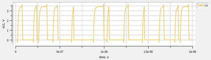
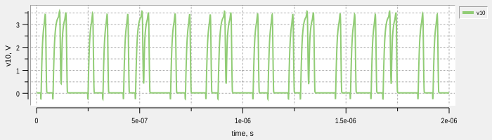
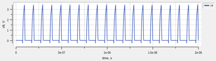
Transient simulation of four-bit adder

This example, like the previous one, involves a circuit run in transient analysis. However, it differs in terms of complexity and the presence of nested subcircuit elements.

The circuit is a classic adder with 2 four-bit inputs, sourced from Ngspice tests (/tests/transient/fourbitadder.cir). We incrementally build it from the simplest NAND logic blocks up to the four-bit adder circuit.

The NAND block itself is constructed from a combination of bipolar transistors, diodes, and resistors. Its definition is as follows:

oo::class create NAND {
    superclass Subcircuit
    constructor {} {
        # define external pins of subcircuit
        set pins {1 2 3 4}
        # define input parameters of subcircuit
        set params {}
        # add elements to subcircuit definition
        my add [Q new 1 9 5 1 -model qmod] [D new 1clamp 0 1 -model dmod] [Q new 2 9 5 2 -model qmod]\
                [D new 2clamp 0 2 -model dmod] [R new b 4 5 -r 4e3] [R new 1 4 6 -r 1.6e3] [Q new 3 6 9 8 -model qmod]\
                [R new 2 8 0 -r 1e3] [R new c 4 7 -r 130] [Q new 4 7 6 10 -model qmod] [D new vbedrop 10 3 -model dmod]\
                [Q new 5 3 8 0 -model qmod]
        # pass name, list of pins and list of parameters to Subcircuit constructor
        next nand $pins $params
    }
}
# create NAND subcircuit definition instance
set nand [NAND new]

To build one-bit adder we use combination of NAND subcircuits:

oo::class create ONEBIT {
    superclass Subcircuit
    constructor {} {
        # define external pins of subcircuit
        set pins {1 2 3 4 5 6}
        # define input parameters of subcircuit
        set params {}
        # add elements to subcircuit definition
        global variable nand
        my add [XAuto new $nand x1 {1 2 7 6}] [XAuto new $nand x2 {1 7 8 6}] [XAuto new $nand x3 {2 7 9 6}]\
                [XAuto new $nand x4 {8 9 10 6}] [XAuto new $nand x5 {3 10 11 6}] [XAuto new $nand x6 {3 11 12 6}]\
                [XAuto new $nand x7 {10 11 13 6}] [XAuto new $nand x8 {12 13 4 6}] [XAuto new $nand x9 {11 7 5 6}]
        # pass name, list of pins and list of parameters to Subcircuit constructor
        next onebit $pins $params
    }
}
# create ONEBIT subcircuit definition instance
set onebit [ONEBIT new]

Previously, we built subcircuits, but here we demonstrate that subcircuits can be used within the definitions of other subcircuits, allowing us to create a multi-level hierarchy for building complex circuits. We start by combining one-bit adders to form two-bit adders, and then increase the level of grouping by connecting two two-bit subcircuits to create a four-bit adder:

oo::class create TWOBIT {
    superclass Subcircuit
    constructor {} {
        # define external pins of subcircuit
        set pins {1 2 3 4 5 6 7 8 9}
        # define input parameters of subcircuit
        set params {}
        # add elements to subcircuit definition
        global variable onebit
        my add [XAuto new $onebit x1 {1 2 7 5 10 9}] [XAuto new $onebit x2 {3 4 10 6 8 9}]
        # pass name, list of pins and list of parameters to Subcircuit constructor
        next twobit $pins $params
    }
}
# create TWOBIT subcircuit definition instance
set twobit [TWOBIT new]

### create class that represents FOURBIT subcircuit
oo::class create FOURBIT {
    superclass Subcircuit
    constructor {} {
        # define external pins of subcircuit
        set pins {1 2 3 4 5 6 7 8 9 10 11 12 13 14 15}
        # define input parameters of subcircuit
        set params {}
        # add elements to subcircuit definition
        global variable twobit
        my add [XAuto new $twobit x1 {1 2 3 4 9 10 13 16 15}] [XAuto new $twobit x2 {5 6 7 8 11 12 16 14 15}]
        # pass name, list of pins and list of parameters to Subcircuit constructor
        next fourbit $pins $params
    }
}
# create FOURBIT subcircuit definition instance
set fourbit [FOURBIT new]

Next step is to initialize top circuit and add all subcircuit definitions to it:

set circuit [Circuit new {Four-bit adder}]
# add elements to circuit
$circuit add [Tran new -tstep 1e-9 -tstop 2e-6]
$circuit add [Options new {{noacct -sw}}]
$circuit add $nand $onebit $twobit $fourbit
$circuit add [XAuto new $fourbit x18 {1 2 3 4 5 6 7 8 9 10 11 12 0 13 99}]

To properly see the circuit in action we define input signals to all eight inputs, as well as power:

set trtf 10e-9
set tonStep 10e-9
set perStep 50e-9
$circuit add [Vdc new cc 99 0 -dc 5]
set i 1
foreach name [list in1a in1b in2a in2b in3a in3b in4a in4b] {
    $circuit add [Vpulse new $name $i 0 -low 0 -high 3 -td 0 -tf $trtf -tr $trtf -pw [expr {$tonStep*pow(2,$i-1)}]\
                          -per [expr {$perStep*pow(2,$i-1)}]]
    incr i
}

Add load resistors:

$circuit add [R new bit0 9 0 -r 1e3] [R new bit1 10 0 -r 1e3] [R new bit2 11 0 -r 1e3] [R new bit3 12 0 -r 1e3]\
        [R new cout 13 0 -r 1e3]

Add semiconductor devices models:

$circuit add [DiodeModel new dmod] [BjtGPModel new qmod npn -bf 75 -rb 100 -cje 1e-12 -cjc 3e-12]

Now we can create simulator and run circuit:

if {[catch {set simulator [Shared new shared1]}]} {
    set simulator [Batch new batch1]
}
# attach simulator object to circuit
$circuit configure -simulator $simulator
# run circuit, read log and data
$circuit runAndRead -vector

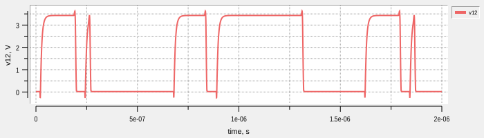
Finally we read the data and plot it as usual:

set data [$circuit getDataDict]
set time [dict get $data time]
set v9 [dict get $data v(9)]
set v10 [dict get $data v(10)]
set v11 [dict get $data v(11)]
set v12 [dict get $data v(12)]

set timeV9 [transpose [list [$time index :] [$v9 index :]]]
set timeV10 [transpose [list [$time index :] [$v10 index :]]]
set timeV11 [transpose [list [$time index :] [$v11 index :]]]
set timeV12 [transpose [list [$time index :] [$v12  index :]]]

### plot data with ticklecharts
set numberFormat [ticklecharts::jsfunc new {
    function (value) {
        return Number(value).toPrecision(2);
    }
}]
set nodes {9 10 11 12}
set layout [ticklecharts::Gridlayout new]
set i -1
foreach node $nodes {
    ticklecharts::chart create chartV$node
    chartV$node SetOptions -title {} -tooltip [list trigger axis valueFormatter $numberFormat] -animation False\
            -toolbox {feature {dataZoom {yAxisIndex none}}}
    chartV$node Xaxis -name {time, s} -minorTick {show True} -type value -splitLine {show True}
    chartV$node Yaxis -name "v(${node}), V" -minorTick {show True} -type value -splitLine {show True}
    chartV$node Add lineSeries -data [set timeV$node] -showAllSymbol nothing -name V(${node}) -symbolSize 0
    $layout Add chartV$node -bottom [expr {4+24*[incr i]}]% -height 18% -width 80%
}
set fbasename [file rootname [file tail [info script]]]
$layout Render -outfile [file normalize [file join .. html_charts $fbasename.html]] -width 800px -height 500px\
        -divid $fbasename -jschartvar chart_$fbasename -jsvar option_$fbasename

Results:

If rbc package is installed, plotting could be done with it:

if {![catch {package require rbc::graphtoolbar}]} {

    set currentDir [file dirname [file normalize [info script]]]
    source [file join $currentDir .. .. common.tcl]
    set i -1
    set nodes {v9 v10 v11 v12}
    foreach node $nodes {
        set graphName .g$node
        rbc::graphtoolbar $graphName -width 700 -height 200 -type graph -controlmode context -zoom -crosshairs\
                -crosshairsmode closest  -pan -zoomwheel
        $graphName graph grid on
        $graphName graph axis configure x -title {time, s}
        $graphName graph axis configure y -title "${node}, V"
        $graphName graph element create $node -x $time -y [set $node] -symbol {} -label $node\
                -color [lindex $colors [incr i]] -linewidth 2
        grid $graphName -row $i -sticky nsew
        grid rowconfigure . $i -weight 1
        lappend members [list [$graphName subwidget graph] x]
        dict set ::axesStates [$graphName subwidget graph] x [$graphName graph axis limits x]
    }
    # A graph may contain several group members; bind it only once.
    foreach graph [lmap member $members {lindex $member 0}] {
        bind $graph  <<RbcAxisLimitsChanged>> [list syncAxisGroup $members %W %d]
    }
    grid columnconfigure . 0 -weight 1
    foreach node $nodes {
        .g$node graph svg output\
                [file normalize [file join .. .. .. docs assets img svg_charts ngspice ${fbasename}_$node.svg]]
    }
}

S-parameter simulation of pass-band filter

This example demonstrates capability of AC simulation with S-parameter output in Ngspice. As the circuit of interest we use band pass filter sourced from Ngspice examples (/examples/sp/filter.sp).

The circuit image is (from Novarianti, Dini. (2019). Design and Implementation of Chebyshev Band Pass Filter with M-Derived Section in Frequency Band 88 - 108 MHz).

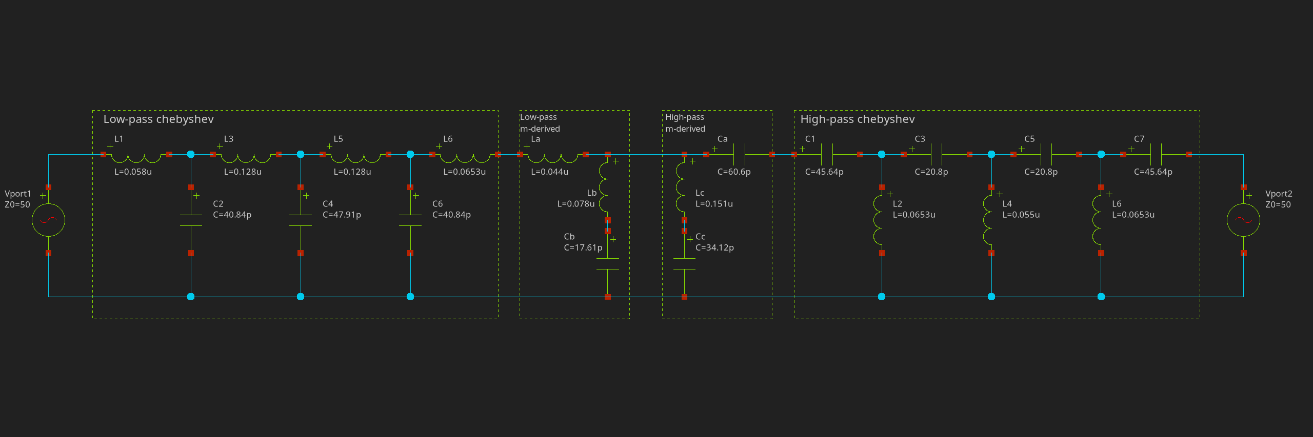
The circuit is built with following code:

set circuit [Circuit new {filter s-parameters}]
# add elements to circuit
$circuit add [Vport new gen 1 0 -dc 0 -ac 1 -portnum 1]
# lowpass Chebyshev
$circuit add [L new 1 1 2 -l 0.058u] [C new 2 2 0 -c 40.84p] [L new 3 2 3 -l 0.128u] [C new 4 3 0 -c 47.91p]\
        [L new 5 3 4 -l 0.128u] [C new 6 4 0 -c 40.48p] [L new 7 4 5 -l 0.0653u]
# lowpass m-derived
$circuit add [L new a 5 6 -l 0.044u] [L new b 6 a -l 0.078u] [C new b a 0 -c 17.61p]
# highpass m-derived
$circuit add [C new a 6 7 -c 60.6p] [L new c 6 b -l 0.151u] [C new c b 0 -c 34.12p]
# highpass Chebyshev
$circuit add [C new 1 7 8 -c 45.64p] [L new 2 8 0 -l 0.0653u] [C new 3 8 9 -c 20.8p] [L new 4 9 0 -l 0.055u]\
        [C new 5 9 10 -c 20.8p] [L new 6 10 0 -l 0.0653u] [C new 7 10 out -c 45.64p]
$circuit add [Vport new l out 0 -dc 0 -ac 0 -portnum 2]
$circuit add [Sp new -variation lin -n 500 -fstart 10meg -fstop 200meg]

You should draw attention to special voltage sources, ::SpiceGenTcl::Ngspice::Sources::Vport, that represents RF-port with special parameter -portnum as a port number, so digits in S-parameters are refered to these port numbers (i.e. S11, S12, S21, S22).

Special analysis object for S-parameter simulation is ::SpiceGenTcl::Ngspice::Analyses::Sp, parameters are the same as for AC analysis:

$circuit add [Sp new -variation lin -n 500 -fstart 10meg -fstop 200meg]

As usual, we create simulator, run the circuit and read the data:

if {[catch {set simulator [Shared new shared1]}]} {
    set simulator [Batch new batch1]
}
# attach simulator object to circuit
$circuit configure -simulator $simulator
$circuit runAndRead -vector
# get data object
set data [$circuit getDataDict]

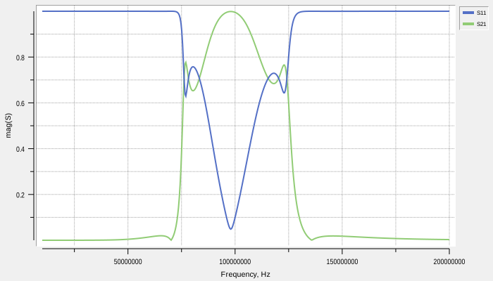
Next few lines of code is used to extract magnitude of S11 and S21 parameters:

vector create freq
freq expr {real([dict get $data frequency])}
# and calculate magnitude of S11 and S21
vector create s11Mag s21Mag
s11Mag expr {abs([dict get $data s_1_1])}
s21Mag expr {abs([dict get $data s_2_1])}

Now we are ready to plot data:

set chart [ticklecharts::chart new]
set numberFormat [ticklecharts::jsfunc new {
    function (value) {
        return Number(value).toPrecision(4);
    }
}]
$chart Xaxis -name {Frequency, Hz} -minorTick {show True} -type value -splitLine {show True}
$chart Yaxis -name mag(S) -minorTick {show True} -type value -splitLine {show True}
$chart SetOptions -title {} -tooltip [list trigger axis valueFormatter $numberFormat] -legend {} -animation False\
        -toolbox {feature {dataZoom {yAxisIndex none}}}
$chart Add lineSeries -data [transpose [list [freq index :] [s11Mag index :]]] -showAllSymbol nothing -name S11\
        -symbolSize 0
$chart Add lineSeries -data [transpose [list [freq index :] [s21Mag index :]]] -showAllSymbol nothing -name S21\
        -symbolSize 0
set fbasename [file rootname [file tail [info script]]]
$chart Render -outfile [file normalize [file join .. html_charts $fbasename.html]] -width 800px -height 500px\
        -divid $fbasename -jschartvar chart_$fbasename -jsvar option_$fbasename

The result is:

On the picture We can clearly see the band that spans from 70Mhz to 135Mhz.

If rbc package is installed, plotting could be done with it:

if {![catch {package require rbc::graphtoolbar}]} {
    set colors {#5470c6 #91cc75}
    set graph [rbc::graphtoolbar .g -width 700 -height 400 -type graph -controlmode context -zoom -crosshairs\
                       -crosshairsmode closest -crosshairsclosestopts {-interpolate no} -pan -zoomwheel -scaletoggle y\
                       -activelegend]
    $graph graph grid on
    $graph graph axis configure x -title {Frequency, Hz}
    $graph graph axis configure y -title mag(S)
    $graph graph element create s11 -x freq -y s11Mag -symbol {} -label S11 -color [lindex $colors 0] -linewidth 2
    $graph graph element create s21 -x freq -y s21Mag -symbol {} -label S21 -color [lindex $colors 1] -linewidth 2
    grid $graph -sticky nsew
    grid columnconfigure . 0 -weight 1
    grid rowconfigure . 0 -weight 1
    $graph graph svg output [file normalize [file join .. .. .. docs assets img svg_charts ngspice $fbasename.svg]]
}

---

Copyright (c) George Yashin